In this post, we will use D2xlab to explore a real IMU (Inertial Measurement Unit) dataset and show how simple numerical operators — forward differences, cumulative sums, and FFT filtering — can be combined to derive meaningful mechanical quantities visually and without code.

The goal is not to produce perfect motion reconstruction, but to understand why filtering is often mandatory when working with real-world signals.

Ship Accelerations Dataset

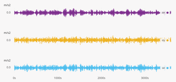
We use a dataset containing 3-axis accelerations (in m/s2) measured onboard a ship moored offshore and subjected to wave excitation.

Once loaded into the D2xlab, we can immediately visualize the three acceleration components in the time history plot. At first glance, the signals look rather smooth — although a closer inspection reveals the presence of high-frequency noise.

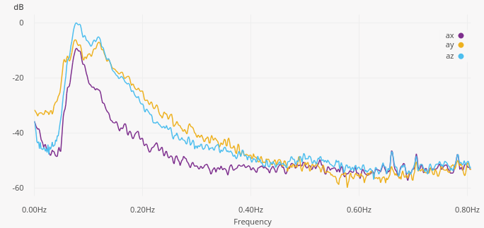
To better understand the signal content, let’s look at the Power Spectral Density. We can see that all three axes exhibit a dominant peak around 0.08 Hz, which most likely corresponds to the dominant wave frequency at the measurement location.

Deriving Velocities and Motions

From acceleration measurments, velocity and position can be estimated through numerical integration. D2xlab provides a cumulative sum operator, which acts as a simple numerical integrator.

Let’s derive the vertical velocity and displacement:

1. Create a new series in the explorer by clicking on the Lightning icon  .
2. Rename it by Right-Click > Rename into vz.
3. In the Calculator Panel enter the formulae cumsum(az) / fs (fs is the reserved keyword for the sampling frequency).
4. Repeat the same process to create a z position series, entering cumsum(vz) / fs for its formulae.

Now inspect the Time History of the vertical z position: it quickly diverges. Did the ship sink :-)?

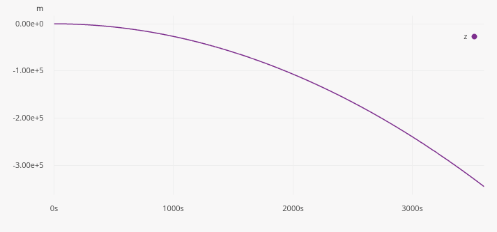
This is a classic result familiar to anyone working with IMUs: tiny sensor biases and small low-frequency errors lead to catastrophic drift after double integration.

So what’s the solution? Filtering.

Removing Drift with Frequency-Domain Filtering

To remove the low-frequency drift, we apply a high-pass FFT filter:

1. Create a new High Pass Filter in the FFT Filter panel and set its frequency around 0.05Hz.
2. Select the velocity signal vz.
3. Activate the FFT Filter in its filter settings

The effect is immediate. Both velocity (vz) and postions (z) now look physically plausible, with the long-term drift removed. You can experiment with the cut-off frequency and directly observe how it impacts the derived motion.

Going The Other Way: Estimating Derivatives

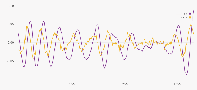
D2xlab also provides a first-order difference operator, which acts as a simple numerical derivative. Let’s estimate the jerk, the derivative of acceleration, using diff(ax) * fs.

We can see that a lot of high frequency noise is created. Numerical differentiation strongly amplifies noise, even when the original signal looks smooth. Applying a low-pass FFT filter to the jerk signal significantly improves readability. By adjusting the cut-off frequency, you can directly see the trade-off between noise reduction and signal fidelity.

Conclusion

This short example highlights several important realities of working with measured signals, including numerical noise, integration drift, and the need for appropriate filtering.

D2xlab does not aim to provide symbolic calculus or perfect motion reconstruction. Instead, it focuses on practical, engineer-grade numerical tools that allow you to explore data quickly, test assumptions, and understand failure modes early — without writing code.

When working with real signals, seeing the problem is often the first step toward solving it!